
Strategy Seasonality Analysis
Seasonality Analysis
Background
- AiLA strategies are classified as based on seasonality, event-driven and Trade flow
- AILA Seasonal strategies include seasonal constituents and non-seasonal constituents
- Seasonal constituents are characterized by price variations driven either by supply variation or demand variations over a 12-16 month cycle
- Commodities with a price variation over a longer economic cycle are considered as Non-Seasonal
- For the purpose of this analysis, we have categorized sector constituents as below
- Seasonal: Agriculture, Oil and Gas
- Non-Seasonal: Base and Precious Metals
Key Questions
- Do seasonal constituents indeed provide an edge in terms of risk adjusted performance?
- What is impact on the overall performance by combining Seasonal and Non-Seasonal constituents in a single strategy?
- Do Non-Seasonal constituents degrade overall performance?
Approach
- AILAF010 Seasonal and diversified long/short global commodity strategy is used for the analysis
- The individual daily return streams from the strategy over the period Jan 2017 - Jan 2026 are grouped in the following order
Seasonal
| Chicago Soybeans | US Arabica Coffee | US WTI |
| Chicago Bean Oil | US Cocoa | US RBOB |
| Chicago Corn | US Cotton | US Heating Oil |
| Chicago Wheat | US Sugar | London Brent |
| Chicago Soy Meal | EU Emissions | London Gas Oil |
| Kansas Wheat | Dutch TTF | US Natural Gas |
| Minneapolis Wheat | UK NBP |
Non-Seasonal
| US Gold | London Aluminium | US Copper |
| US Silver | London Lead | London Zinc |
| US Platinum | US Palladium |
The two return streams form the basis for the analysis
Performance Comparison
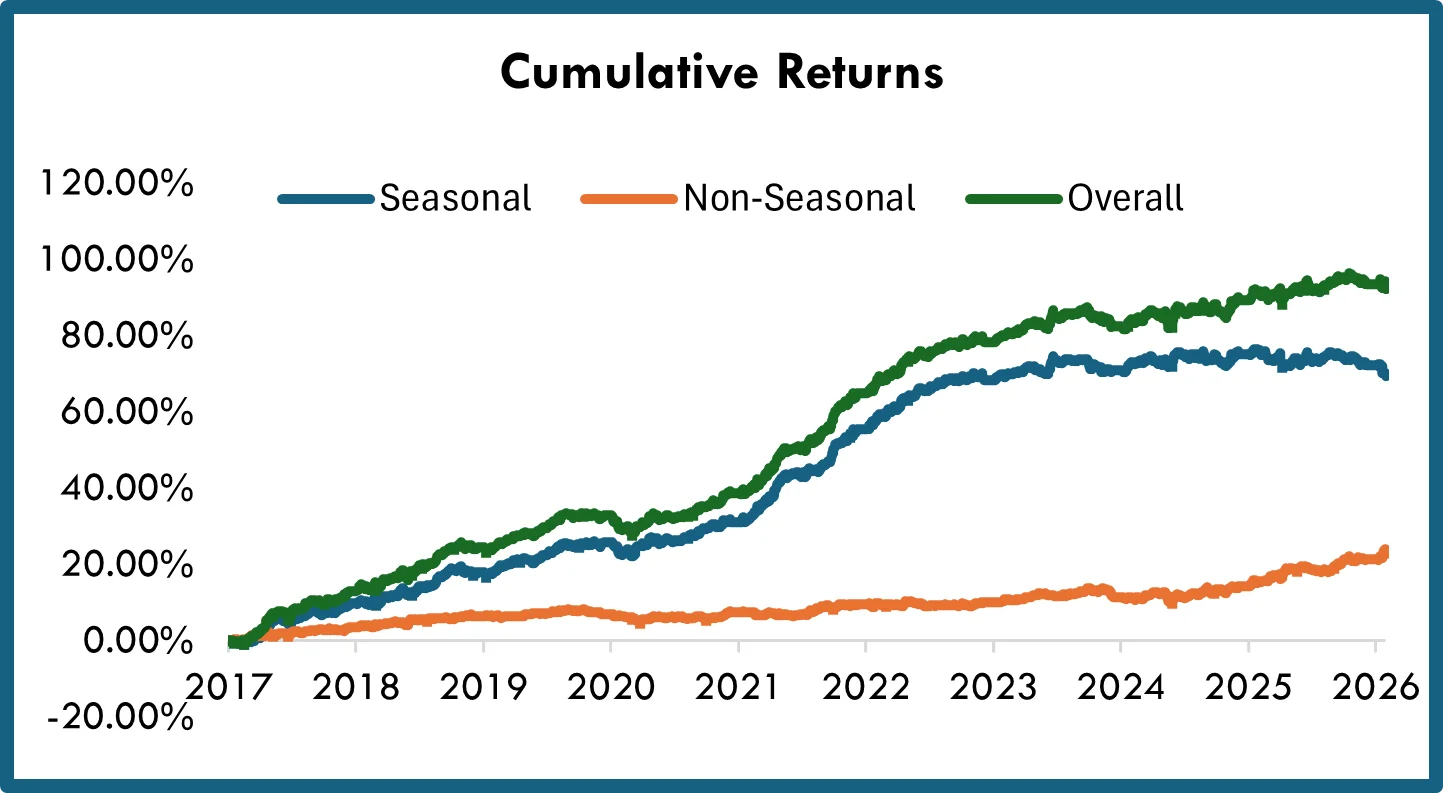
- Cumulative returns are compared across the entire period from Jan 2017 to Jan 2026
- As observed, the Seasonal group is the main contributor to the overall strategy returns which is primarily on account of larger number of constituents
- The seasonal group additionally benefits from diversity across sectors and regions while the Non-Seasonal group is concentrated in Metals
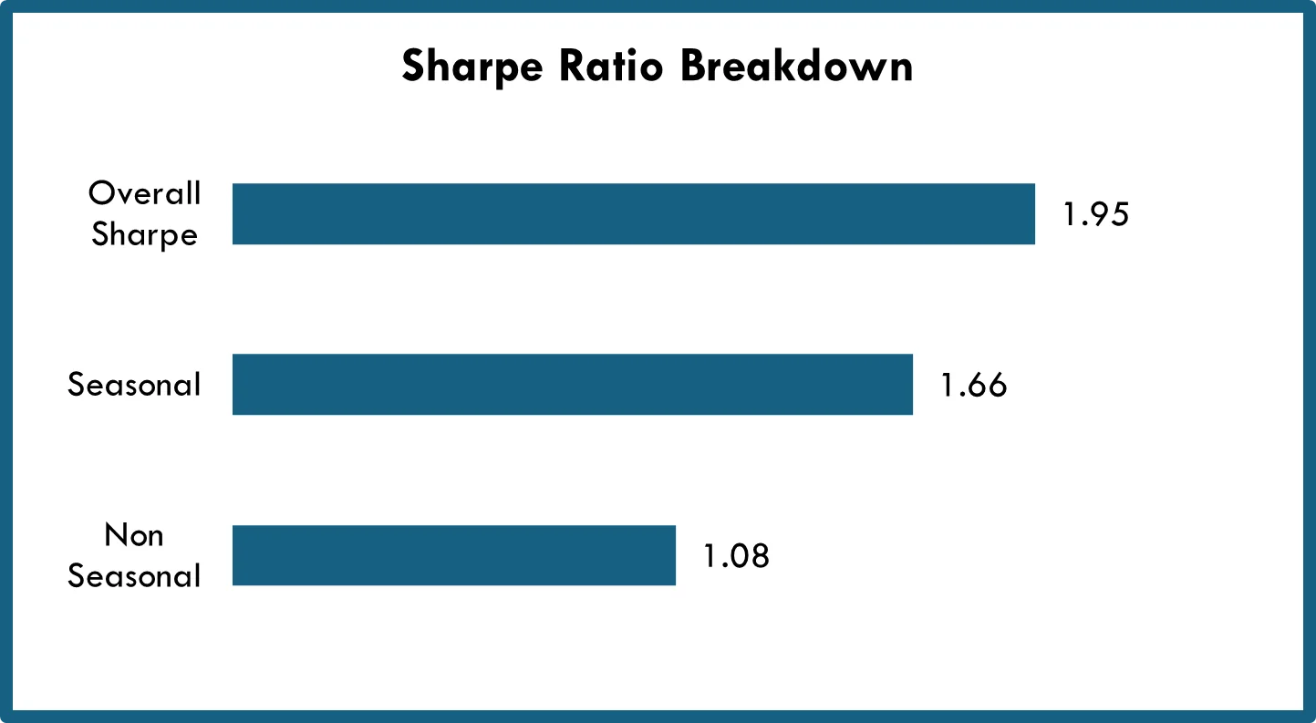
- Sharpe ratio is a better metric to compare the risk adjusted performance of the two groups
- From the adjacent figure we see that Seasonal has a higher Sharpe ratio (1.66) in comparison to Non-Seasonal (1.08)
- The Sharpe Ratio of the overall strategy is however better than both the groups implying a complementary impact between the two groups
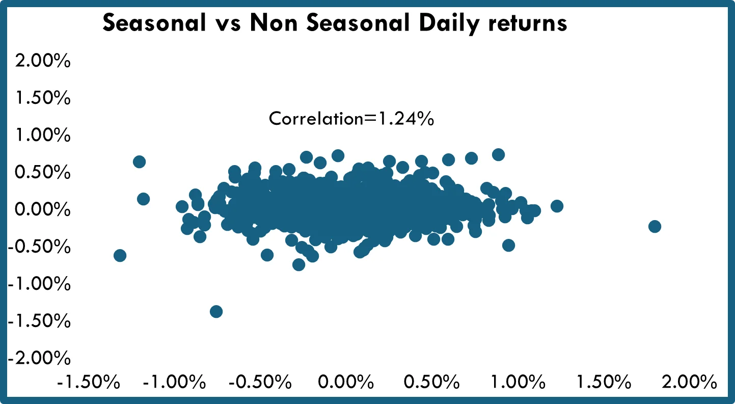
- To further understand the impact between the groups, the correlation between the daily return streams groups was examined
- As observed from the chart there is a very insignificant correlation between the two groups (Correlation = 1.24%)
- This implies that the Non-Seasonal group reduces the volatility in the overall portfolio, also provides an explanation for the improved Sharpe ratio of the overall portfolio
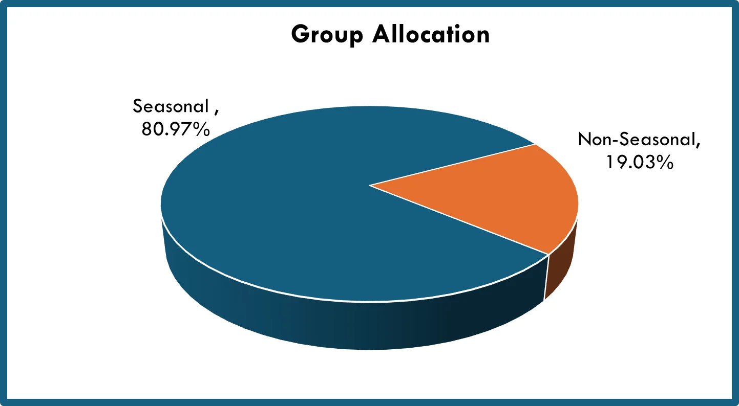
- Another factor examined is the breakdown of the capacity allocation between the groups (Seasonal: 80.97%, Non-Seasonal: 19.03%)
- The low correlation and the complementary impact implies that the inclusion of Non-Seasonal constituents in the strategy provides opportunities to enhance the allocation capacity
Conclusions
- Seasonal constituent group is the primary performance driver for the portfolio providing consistent returns over the period with an overall Sharpe ratio of 1.66
- Non-Seasonal group underperforms the Seasonal group and has a lower Sharpe ratio of 1.08
- There is insignificant correlation between the return streams
- The performance and Sharpe ratio of the overall strategy, performs better than either of the two seasonal and non-seasonal with higher Sharpe ratio of 1.95
- This implies the Non-Seasonal constituents complement the Seasonal constituents in having a favorable impact on the overall return and risk profile of the strategy
- This favorable impact can be attributed to
- Reduced portfolio volatility because of low correlation between the Seasonal and Non-Seasonal group return streams
- Non-Seasonal providing enhanced allocation capacity to the strategy further reducing volatility